HMC Igor Procedure Help File
The Igor code in the HMC.ipf procedure file will produce the HMC menu and supply the commands listed below. You can download a copy of this procedure file from this page.
Fix Graph (Command-2)
Adjust the settings of the front-most graph, assuming that the data should be plotted as discrete points, axes mirrored, ticks inward, and no standoff. This command also adjusts the font and font size. Call this function before you attempt a fit.
Add ChiSq Information (Command-3)
Run this command immediately after you perform a weighted nonlinear least-squares fit, provided that you have requested a textbox with fitting information be added to the graph. You make that selection in the fourth tab of the Curve Fitting… dialog. Also make sure to select Auto Trace from the Residuals popup and check the box Fit Function Name in TextBox Preferences...
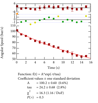
Normalized Residuals (Command-F3)
If you wish to add a panel of normalized residuals (the residual divided by the uncertainty for each data point), issue this command after a fit. A panel of normalized residuals will be inserted between the residuals and the data, as shown in the graph below. The normalized residuals will be color coded to indicate their magnitude.
Date Notes (Command-4)
Open up (or bring to the front) a formatted notebook window for taking lab notes, and append a line with the current date and time. You can type into this window, paste graphs and other pictures. If you want your pasted graphs to be viewable on both Macs and PCs, use the PNG format. You can set this format using the Export Graphics command from the Edit menu. Once you set it, that’s the format that will be used on subsequent Copy operations.
Sample Variance (Command-5)
This command requires that you are running Igor Version 6.2 or later.
If you are taking several measurements of a dependent variable at each value of an independent variable, this command can make your life much more efficient and reduce the need to toggle back and forth between Igor and Excel. Suppose, for example, that you are measuring the time of flight of a projectile as a function of the launch angle. You will take several trials at each angle (the independent variable) and wish to use the average and standard error of the times (the dependent variable) for each angle.
Issue the Sample Variance command and enter Launch_Angle for the independent variable name, and Flight_Time for the dependent variable name. Note: these names must not contain spaces or other punctuation, other than underscores. If they are not unique, you will be asked whether to overwrite previous data. If you don't wish to lose prior data, you must use a new name for both the independent and dependent variables.
Once you have entered satisfactory variable names, you will see a panel similar to the one shown below.
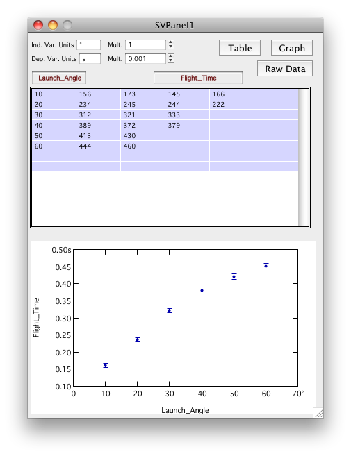
The units of the independent variable are degrees, which may be entered as option-shift-8 on a Macintosh. The dependent variable is measured in milliseconds, but in Igor it is preferable to use the base SI unit of seconds. I have therefore entered a multiplier of 0.001, so that the values in the raw table may be typed without decimal points.
The left-most column holds the values of the independent variable (the launch angle), while the remaining columns to the right hold values for the dependent variable (the flight time). As data are entered, the plot beneath the table is updated. The error bars shown in the figure are the standard error computed from the points in the table. Each time a value is updated, so are the average and standard error. Empty cells are not counted.
Clicking on the Table button brings up a table of the averages and standard errors. Clicking on the Graph button produces a new graph window similar to the graph at the bottom of the Panel, but more convenient for you to use for fitting operations.