Using a Spreadsheet
Spreadsheets are very handy for manipulating and visualizing data. They facilitate repetitive calculations and allow you to keep track of the operations you have made. They can also plot results, and can be made to update the plots whenever you change or add to your data. Spreadsheets are typically not particularly good at making final graphs of data, or in performing powerful “curve fitting” operations on data. For these tasks, use a dedicated plotting and data analysis program, such as Igor Pro. Using Microsoft Excel you can quickly compute the mean, standard deviation, and standard deviation of the mean (SDOM) of a set of data, and you can rapidly perform all sorts of error calculations.
Computing Means and Standard Deviations
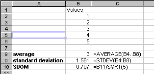
A common task is to average several data points, and compute the standard deviation of the mean (SDOM) to estimate the uncertainty of the measurement. The figure shows an example of performing this calculation. The values to average are placed in column B, rows 2 through 5. In cell B8 a formula is typed to compute the mean (average). The formula is shown immediately to the right. It is =AVERAGE(B4..B8). All formulas in Excel begin with an equal sign, which must be the first character in the formula. The argument to the AVERAGE function is a range of cells. Of course, for this example you can calculate the mean by inspection, but it's reassuring that Excel gets the right answer.
The next cell down has the formula for computing the standard deviation. Does Excel use \( N \) or \( N - 1 \) to compute the standard deviation? Is the computation of the SDOM done correctly?
Repetitive Calculations
Even better than computing something once using Excel is reusing the calculation many times. If you have a great many sets of 5 numbers for which you need to know the statistics, you can just type the new values over the 5 old values and write down the resulting average and SDOM. Alternatively, you can type each set of values in its own column and copy the formulas for average, standard deviation, and SDOM from column B to all the other columns.
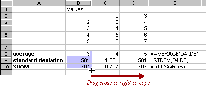
Select the cells whose formulas you wish to copy (B8..B10). Then place the cursor at the lower right corner of cell B10. It will turn from an arrow to the solid black cross shown. Drag to the right through two columns and updated formulas will be written into these two columns. The average of each successive column has indeed risen by 1, as it should. Note also that the formula in D8, as shown in E8, now involves the values in column D, not column B as in the source. Excel automatically updates the references. Cell references that are modified when copied in this way are called relative references. Why are the standard deviation and SDOM values the same?
Plotting Data as You Go
Excel is also very useful for entering and plotting data as you take it. Making a crude plot as you go is a very useful way to see whether the data make sense, where you might need to take more points, and when a data point doesn't seem to be following the trend. Can you spot the errant point in the data sheet and plot below?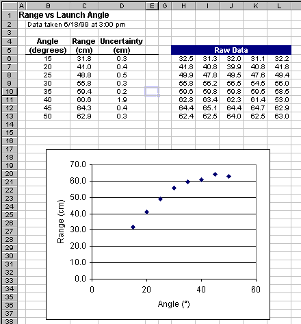
Here’s how to put together such a sheet.
- Label the data sheet with an informative title that explains what data you are taking and when.
- Enter the titles for the columns you need. You can adjust their formatting with the icons in the toolbar, if you like. Although the raw data come logically before their mean and SDOM, I find it more convenient to put the raw data to the right, leaving room for the results you really care about.
- Set up the formulas for the first row. In this case, the raw data are separate trial values for the range (in centimeters). To get the best estimate of the true range, we average using Excel's AVERAGE function. In cell C6 use the formula =AVERAGE($H6..$L6). The dollar signs make the column references absolute, so they won't change when you copy.
- Copy this formula to cell D6 either using Copy and Paste or by dragging the box at the lower right corner of cell C6. Then edit the formula, changing the word AVERAGE to STDEV, then appending the text /SQRT(5) so the whole formula reads =STDEV($H6..$L6)/SQRT(5). This computes the standard deviation of the mean (SDOM).
- Now you can select the two formulas you have created and copy them down as many rows as you like. As you type in your experimental values in the Raw Data table, the appropriate averages and uncertainties are immediately recalculated.
- To set up the graph, select cells B6 through C15 (or you can even select more rows, if you expect to take data at more than 10 launch angles). Then click the chart tool button to set up the graph. This kind of graph is called an XY (Scatter) graph. Answer the questions and let Excel put the graph on the page. As you type in more data values, the graph automatically updates. Very nice!